Recently I had to create a figure that concisely compared ten coefficients within each of eight separate models. The models were variations on the primary results reported in a recent Criminology article I co-wrote with Megan Denver about perceptual mediators of criminal record stigma. Long story short, we had two primary sets of results: 1) direct effects and 2) total effects; four randomly assigned treatments (various positive employment credentials), and nine alternative models we needed to compare to our model using the full sample for analysis.
Needless to say, it was a lot to include in one figure but I thought a forest plot – or blobbogram – could come in handy. I’ve seen these used in meta-analyses before and although the current project was not a meta-analysis, it seemed the information contained in a forest plot suited this need well enough.
I first had to load the required libraries, define a font, and populate the coefficient data for the direct effects.
## LOAD LIBRARIES
  my_packages<-c("ggplot2", "gridExtra", "cowplot")
  lapply(my_packages, require, character.only=TRUE)

## DEFINE FONT FOR PLOTS
  windowsFonts(TNR=windowsFont("Times New Roman"))

## CREATE COEFFICIENT DATA FOR FULL MODEL (DIRECT EFFECTS)
  models<-c("Full Sample", "Emp Only", "Depend First", "Depend Last",
            "Recid Risk First", "Recid Risk Last", "Trust First",
            "Trust Last", "Wrkplc Crime First", "Wrkplc Crime Last")
  index<-c(1:10)

## INVOL JOB TRAINING
  invol_ptest<-rev(c(.434, .303, .314, .658, .360, .455, .440, .301, .592, .328))
  invol_se<-rev(c(.105, .162, .217, .224, .216, .205, .220, .219, .226, .221))
  invol_ub<-invol_ptest+(1.96*invol_se)
  invol_lb<-invol_ptest+(-1.96*invol_se)

## VOL JOB TRAINING
  vol_ptest<-rev(c(.722, .844, .813, .893, .711, .717, .607, .762, .848, .721))
  vol_se<-rev(c(.108, .169, .213, .237, .228, .221, .232, .221, .237, .220))
  vol_ub<-vol_ptest+(1.96*vol_se)
  vol_lb<-vol_ptest+(-1.96*vol_se)

## OCCUP LICENSE
  occup_ptest<-rev(c(.556, .541, .294, .842, .676, .645, .577, .356, .836, .471))
  occup_se<-rev(c(.104, .162, .230, .209, .221, .205, .222, .240, .209, .229))
  occup_ub<-occup_ptest+(1.96*occup_se)
  occup_lb<-occup_ptest+(-1.96*occup_se)

## REF LETTER
  reflet_ptest<-rev(c(1.145, 1.231, 1.044, 1.119, 1.391, 1.400, .969, 1.182, 1.302, 1.090))
  reflet_se<-rev(c(.113, .175, .234, .238, .233, .239, .232, .236, .253, .235))
  reflet_ub<-reflet_ptest+(1.96*reflet_se)
  reflet_lb<-reflet_ptest+(-1.96*reflet_se)

## ADD ALL VARS TO DATA FRAME
  drtfx<-data.frame(models, invol_ptest, invol_se, invol_ub, invol_lb,
                    vol_ptest, vol_se, vol_ub, vol_lb,
                    occup_ptest, occup_se, occup_ub, occup_lb,
                    reflet_ptest, reflet_se, reflet_ub, reflet_lb)
That accomplished, I then created the individual plots for the direct effects.
## INVOL JOB TRAINING
  invol_drtfx<-ggplot(drtfx, aes(y=index, x=invol_ptest, xmin=invol_lb,
                            xmax=invol_ub)) +
    geom_point() +
    geom_errorbarh(height=.1) +
    scale_y_continuous(name="", breaks=1:length(drtfx$invol_ptest),
                       labels=rev(models)) +
    geom_vline(xintercept=drtfx$invol_ub[10], linetype='dashed') +
    geom_vline(xintercept=drtfx$invol_lb[10], linetype='dashed') +
    ggtitle("Direct Effects") +
    theme(plot.title=element_text(hjust=0.5)) +
    xlab("Involuntary Job Training") +
    theme(text = element_text(family = "TNR"))

## VOL JOB TRAINING
  vol_drtfx<-ggplot(drtfx, aes(y=index, x=vol_ptest, xmin=vol_lb,
                            xmax=vol_ub)) +
    geom_point() +
    geom_errorbarh(height=.1) +
    scale_y_continuous(name="", breaks=1:length(drtfx$vol_ptest),
                       labels=rev(models)) +
    geom_vline(xintercept=drtfx$vol_ub[10], linetype='dashed') +
    geom_vline(xintercept=drtfx$vol_lb[10], linetype='dashed') +
    xlab("Voluntary Job Training") +
    theme(text = element_text(family = "TNR"))

## OCCUPATIONAL LICENSE
  occup_drtfx<-ggplot(drtfx, aes(y=index, x=occup_ptest, xmin=occup_lb,
                            xmax=occup_ub)) +
    geom_point() +
    geom_errorbarh(height=.1) +
    scale_y_continuous(name="", breaks=1:length(drtfx$occup_ptest),
                       labels=rev(models)) +
    geom_vline(xintercept=drtfx$occup_ub[10], linetype='dashed') +
    geom_vline(xintercept=drtfx$occup_lb[10], linetype='dashed') +
    xlab("Occupational License") +
    theme(text = element_text(family = "TNR"))

## REFERENCE LETTER
  reflet_drtfx<-ggplot(drtfx, aes(y=index, x=reflet_ptest, xmin=reflet_lb,
                            xmax=reflet_ub)) +
    geom_point() +
    geom_errorbarh(height=.1) +
    scale_y_continuous(name="", breaks=1:length(drtfx$reflet_ptest),
                       labels=rev(models)) +
    geom_vline(xintercept=drtfx$reflet_ub[10], linetype='dashed') +
    geom_vline(xintercept=drtfx$reflet_lb[10], linetype='dashed') +
    xlab("Reference Letter") +
    theme(text = element_text(family = "TNR"))
I then repeat the same process for the total effects (I use the same object names for sake of simplicity).
## CREATE COEFFICIENT DATA FOR REDUCED MODEL (TOTAL EFFECTS)
  labels<-c("Full Sample", "Emp Only", "Depend First", "Depend Last",
            "Recid Risk First", "Recid Risk Last", "Trust First",
            "Trust Last", "Wrkplc Crime First", "Wrkplc Crime Last")

  ## INVOL JOB TRAINING
    invol_ptest<-rev(c(.737, .751, .666, 1.172, .425, .516, .962, .315, .843, .824))
    invol_se<-rev(c(.105, .171, .218, .229, .216, .206, .220, .221, .226, .221))
    invol_ub<-invol_ptest+(1.96*invol_se)
    invol_lb<-invol_ptest+(-1.96*invol_se)

  ## VOL JOB TRAINING
    vol_ptest<-rev(c(1.398, 1.574, 1.334, 1.866, 1.547, 1.448, 1.423, 1.162, 1.538,               1.462))
    vol_se<-rev(c(.109, .171, .217, .240, .230, .224, .235, .223, .240, .219))
    vol_ub<-vol_ptest+(1.96*vol_se)
    vol_lb<-vol_ptest+(-1.96*vol_se)

  ## OCCUP LICENSE
    occup_ptest<-rev(c(1.257, 1.435, .897, 1.624, 1.447, 1.282, 1.329, 1.202, 1.486, 1.227))
    occup_se<-rev(c(.105, .162, .228, .215, .223, .204, .226, .241, .210, .229))
    occup_ub<-occup_ptest+(1.96*occup_se)
    occup_lb<-occup_ptest+(-1.96*occup_se)

  ## REF LETTER
    reflet_ptest<-rev(c(3.044, 3.128, 3.078, 3.069, 3.157, 3.615, 3.201, 2.898, 3.126, 3.135))
    reflet_se<-rev(c(.116, .180, .246, .245, .236, .249, .248, .241, .252, .246))
    reflet_ub<-reflet_ptest+(1.96*reflet_se)
    reflet_lb<-reflet_ptest+(-1.96*reflet_se)

## ADD ALL VARS TO DATA FRAME
  ttlfx<-data.frame(invol_ptest, invol_se, invol_ub, invol_lb,
                    vol_ptest, vol_se, vol_ub, vol_lb,
                    occup_ptest, occup_se, occup_ub, occup_lb,
                    reflet_ptest, reflet_se, reflet_ub, reflet_lb,
                    index, labels)

## CREATE AND STORE SEPARATE CONFIDENCE INTERVAL PLOTS
  ## INVOL JOB TRAINING
    invol_ttlfx<-ggplot(ttlfx, aes(y=index, x=invol_ptest, xmin=invol_lb,
                              xmax=invol_ub)) +
      geom_point() +
      geom_errorbarh(height=.1) +
      scale_y_continuous(name="", breaks=1:length(ttlfx$invol_ptest),
                         labels=rev(labels)) +
      geom_vline(xintercept=ttlfx$invol_ub[10], linetype='dashed') +
      geom_vline(xintercept=ttlfx$invol_lb[10], linetype='dashed') +
      theme(axis.text.y=element_blank(),
            axis.ticks.y=element_blank()) +
      ggtitle("Total Effects") +
      theme(plot.title=element_text(hjust=0.5)) +
      xlab("Involuntary Job Training") +
      theme(text = element_text(family = "TNR"))

  ## VOL JOB TRAINING
    vol_ttlfx<-ggplot(ttlfx, aes(y=index, x=vol_ptest, xmin=vol_lb,
                            xmax=vol_ub)) +
      geom_point() +
      geom_errorbarh(height=.1) +
      scale_y_continuous(name="", breaks=1:length(ttlfx$vol_ptest),
                         labels=rev(labels)) +
      geom_vline(xintercept=ttlfx$vol_ub[10], linetype='dashed') +
      geom_vline(xintercept=ttlfx$vol_lb[10], linetype='dashed') +
      theme(axis.text.y=element_blank(),
            axis.ticks.y=element_blank()) +
      xlab("Voluntary Job Training") +
      theme(text = element_text(family = "TNR"))

  ## OCCUPATIONAL LICENSE
    occup_ttlfx<-ggplot(ttlfx, aes(y=index, x=occup_ptest, xmin=occup_lb,
                              xmax=occup_ub)) +
      geom_point() +
      geom_errorbarh(height=.1) +
      scale_y_continuous(name="", breaks=1:length(ttlfx$occup_ptest),
                         labels=rev(labels)) +
      geom_vline(xintercept=ttlfx$occup_ub[10], linetype='dashed') +
      geom_vline(xintercept=ttlfx$occup_lb[10], linetype='dashed') +
      theme(axis.text.y=element_blank(),
            axis.ticks.y=element_blank()) +
      xlab("Occupational License") +
      theme(text = element_text(family = "TNR"))

  ## REFERENCE LETTER
    reflet_ttlfx<-ggplot(ttlfx, aes(y=index, x=reflet_ptest, xmin=reflet_lb,
                               xmax=reflet_ub)) +
      geom_point() +
      geom_errorbarh(height=.1) +
      scale_y_continuous(name="", breaks=1:length(ttlfx$reflet_ptest),
                         labels=rev(labels)) +
      geom_vline(xintercept=ttlfx$reflet_ub[10], linetype='dashed') +
      geom_vline(xintercept=ttlfx$reflet_lb[10], linetype='dashed') +
      theme(axis.text.y=element_blank(),
            axis.ticks.y=element_blank()) +
      xlab("Reference Letter") +
      theme(text = element_text(family = "TNR"))
The final step was to combine the plots into a 4X2 grid so that all the coefficients and their 95% confidence intervals could be examined simultaneously:
## COMBINE GRAPHS (COWPLOT)
  plot_grid(invol_drtfx, invol_ttlfx, vol_drtfx, vol_ttlfx, occup_drtfx,
            occup_ttlfx, reflet_drtfx, reflet_ttlfx, ncol=2, nrow=4,
            rel_widths=c(4.25/8, 3.75/8))
The resulting plot looks like this:
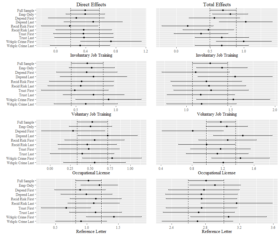
For context, the other candidate models included an employer-only sample of respondents (“Emp Only”) and then eight additional models that varied which mediating question was asked first/last. For additional details about these models, please see my Research Gate page for this publication (there’s a free preprint to download there, too).
So, what does the figure tell me about the comparability of the results? Using the first row of each subgraph as the comparison (“Full Sample”), I can see that most point estimates lie within the confidence interval about the main treatment effect results for each of the types of positive credentials and effect (Direct/Total) under consideration. Even if the point estimates don’t lie within the main confidence interval, all confidence intervals at least overlap slightly with the interval for the main treatment effect using the full sample.
One thing that Megan and I did take notice of was the wide amount of variation for the Involuntary Job Training credential for its various estimates of the total effect. Though they are all comparable to the main effect of interest, we found it interesting that the effects varied so much above and below the confidence interval for the full sample. We surmise this is because the Involuntary Job Training credential presents a difficult-to-interpret signal in the employment context – while it verifies an applicant has a standard set of skills, it also conveys that they were assigned to this program by a judge. The respondents in our study took very different information from this credential and this varied slightly (though not enough to be worrisome) depending upon which mediator questions they were asked first or last. Under normal circumstances, I’d be worried about how the information about the credential was conveyed to respondents but, considering that other research also suggests that involuntary credentials are weak (even negative) labor market signals, I think these results indicate that it’s not easy to interpret a credential when the person with said credential didn’t have agency in deciding to participate in a program.
All this being said, the above figure is nestled at the end of an online appendix that very few people will ever read, so I just wanted to write a post about it because I found its construction and the results interesting!